-JustDoIt-Nike-Tweets
Nike #JustDoIt Marketing Campaign Tweets Dataset: Project Overview (https://nrolle.github.io/-JustDoIt-Nike-Tweets/)
- Wrangled and tokenized the text of 5,000 tweets
- Visualized word counts using word clouds and bar graphs
- Performed sentiment analysis to identify the overall emotion of the text
This is a case study surrounding a marketing campaign conducted by Nike back in 2018. The dataset contains approximately 5,000 tweets in response to the marketing campaign. This particular marketing campaign is significant to me because it marked the day that Nike publicly stood with athlete and activist Colin Kaepernick in his efforts to bring attention to police brutality and the mistreatment of black and brown people in the United States. The objective of this project is to gain some insight in how the public reacted to Nike’s marketing campaign. I will be accomplishing this through tokenzing the text, sentiment analysis, and some graphical and numerical summaries of the dataset.
Code and Resources Used
RStudio Version: 1.4.1103 Packages: tidyverse, dplyr, tibble, tidytext, textdata, worldcloud2 Dataset(https://www.kaggle.com/eliasdabbas/5000-justdoit-tweets-dataset?select=justdoit_tweets_2018_09_07_2.csv)
Data Cleaning
- Selected only the columns deseriable for analysis and assigned them into a new data frame
- Removed tweets that did not relate to the topic (for example, renowned actor, Mark Hamill made a tweet using #JustDoIt that had nothing to do with Nike or the marketing campaign)
Removing Stop Words
- Stop words are common words that are not insightful for our analysis (such as the, like, and,etc.)
- Created a data frame composed of custom stop words
- A data frame of common stop words are available in the tidytext package as “stop_words”
- Combined the data frame “stop_words” and my “custom_stop_words”
- This is to ensure that R ignores words that are not insightful in our analysis
Tokenzing the dataset
- Some basic Natural Language Processing (NLP) Vocabulary
- Every unique word is a term
- Every occurrence of a term is a token
- Tokenzing is the process of creating a “bag of words”
- Created a new object that gives us a column with a unique word in each row from each tweet
Counting the words
- Now that we imposed structure to the text we can count the words
Appending NRC Dictionary
- The Tidytext package includes 4 distinct sentiment dictionaries that works to tag each unique word with a sentiment
- I used the “NRC” dictionary to examine the overall emotional valence of the text
- The “NRC” dictionary defines each unique word as either negative, postiive, fear, anger, trust, sadness, disgust, anticipation, joy, or surprise
Sentiment Analysis
- By counting the number of occurreneces for each sentiment, we can get an understanding for the overall emotional valence of the text
- I created a bar graph to visualize what sentiment occurs the most

Top Twitter Handles Mentioned
- I created a data frame that told me what twitter handles were mentioned the most in these tweets
- I used a bar graph to visualize this

Trump, Kaepernick, Nike, Serena Williams
- In the previous bar graph we saw that the top twitter handles mentioned in this data set was Former President Donald Trump, Colin Kaepernick, Nike, and Serena Williams
- I thought it was be interesting to go further and look at the words and sentiment used when twitter users mentioned these influential figures
Trump - Word Cloud & Bar Graph
- I created a word cloud and bar graph to see the language used when twitter users mentioned @realDonaldTrump


Nike - Word Cloud & Bar Graph
- I created a word cloud and bar graph to see the language used when twitter users mentioned @Nike


Serena Williams - Word Cloud & Bar Graph
- I created a word cloud and bar graph to see the language used when twitter users mentioned @serenawilliams


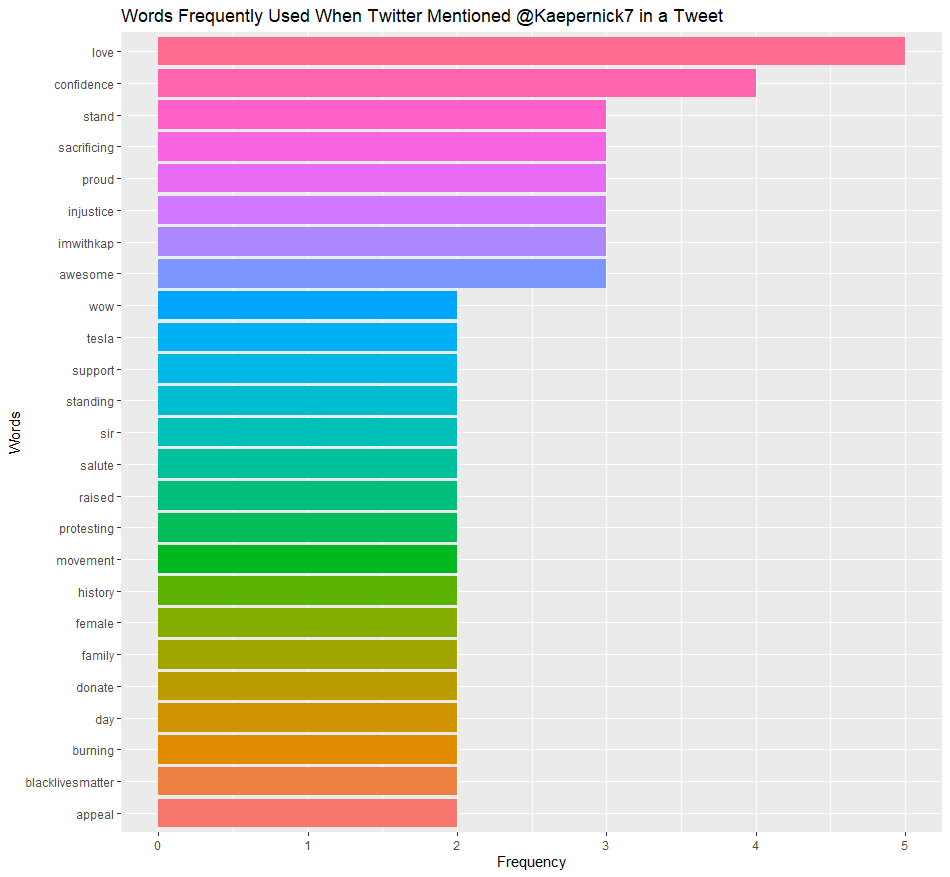
Colin Kaepernick - Word Cloud & Bar Graph
- I created a word cloud and bar graph to see the lagnauge used when twitter users mentioned @Kaepernick7

Conclusion
- This marketing campaign was a successful brand marketing strategy for Nike
- At the time, not many companies had taken a stanceo n the topic of athlete activism in sport. For Nike to take a stance instead of remaining neutral was risky, however, it ultimately resonated well with its ocnsumes and reinforced the brand’s identity
#JustDoIt Case Study
Install necessary packages
install.packages(“tidyverse”) install.packages(“dplyr”) install.packages(“tibble”) install.packages(“tidytext”) install.packages(“textdata”) install.packages(“wordcloud2”)
Setting up the R Environment - Loading Libraries
library(tidyverse) library(dplyr) library(tibble) library(tidytext) library(textdata) library(topicmodels) library(tm) library(wordcloud2)
Read in File
JustDoIt = read.csv(“C:/Users/Nick/Desktop/justdoit_tweets_2018_09_07_2.csv”)
Data Cleaning
Tweets = JustDoIt %>% select(tweet_full_text, user_verified, tweet_retweet_count, tweet_favorite_count, user_screen_name, tweet_in_reply_to_screen_name, user_description, user_followers_count)
Tweets2 = Tweets[-c(1466),]
Number of rows in the Dataset
nrow(Tweets2)
Number of columns in the Dataset
ncol(Tweets2)
Overview of the Dataset
str(Tweets2)
Sample Tweet
sample = Tweets2 %>% select(user_screen_name, tweet_full_text)
sample_n(sample,1)
Removing words that are insigificant to the analysis
custom_stop_words = tribble(~word, “â”,”ðÿ”,”https”,”ï”,”t.co”,”realdonaldtrump”, “thinking”,”amp”,”kaepernick7”,”kaepernick”, “president”,”justdoit”,”nike”,”trump”, “people”,”ºðÿ”,”youâ”,”✔,”takeaknee”,”colinkaepernick”,”donâ”,”theyâ”, “ðÿš”,”potus”,”black”,”job”,”ve”,”shoes”,”white”,”unlike”,”money”,”real”,”weâ”, “wear”,”means”,”message”,”buy”,”stock”,”amendement”,”business”,”america”, “tweet”, “world”,”time”,”american”,”country”,”care”,”americans”,”ˆðÿ‘ÿðÿ”, “attention”,”bought”,”hey”,”canâ”,”ðÿ’ªðÿ”,”iâ”,”idk”,”paid”,”thatâ”, “wearing”,”commercial”, “ad”, “campaign”,”✚ðÿ”,”itâ”,”nikead”,”å”,”athletes”, “justdidit”,”marketing”,”pair”,”bogo”,”朔,”œðÿ”,”ä”,”15”,”ck”,”colin”,”æ”, “advertising”, “cqzvnmockn”,”doesnâ”,”customer”,”kapernick”,”nfl”,”æ”,”apparel”,”ðÿ‘œ”, “ðÿ‘ÿ”,”nikeâ”,”nikecommercial”,”nikestore”,”serenawilliams”,”tonight’s”, “waiting”,”yâ”,”workers”,”weekend”,”taking”,”saturday”,”ðÿž”,”advances”,”7th”, “ceio2wcuyr”,”gkzrtyolqk”,”ll”,”lil”,”olc766xhvz”,”quicker”,”tonightâ”, “womenâ”,”themasb1”,”cutieðÿ’œ”,”ðÿ’ª”,”2”,”5i9egyh9tk”,”paylessinsider”, “payless”,”nflpa”,”nflcommish”,”gbmnyc”,”kstills”, “mosesbread72”,”1jedi_rey”,”havok_2o18”,”theswprincess”,”listentoezra”, “debbieinsideris”,”jeffbfish”,”knot4sharing”,”malcolmjenkins”,”kingjames”, “imwithkaep”, “matthewwolfff”,”kneel”,”jynerso_2017”,”jainaresists”,”b52malmet”, “deadpoolresists”,”debbiesideris”,”jynerso_2017”,”lady_star_gem”,”minervasbard”, “natcookresists”,”rebelscumpixie”,”sabineresists”,”trinityresists”,”drawing”, “batmanresist”,”brandontxneely”,”blue”,”captainslog2o18”,”earl_thomas”,”exercise”, “nateboyer37”,”plays”,”realtomsongs”,”tdlockett12”,”trisresists”,”xtxoan4y7d”, “ybbkaren”,”zmndpufdoh”, “president”,”police”,”football”,”gear”,”lord”,”god”, “military”,”catch”,”school”,”labor”,”wait”,”feeling”,”vote”,”pay”,”deal”,”words”,”coming”, “finally”,”shot”,”chance”,”guess”,”leave”,”change”,”mouth”,”fisa”,”1st”,”1”, “10”,”nikes”,”blah”,”orange”,”buying”,”single”,”anonymous”,”office”,”stuff”, “life”,”kids”,”lie”,”bad”,”btw”,”concept”,”level”,”players”,”kap”, “national”,”serve”,”social”,”sell”,”company”,”true”,”decision”,”watching”,”running”, “guy”,”ooh”,”f45”, “gum”, “chose”,”yr”,”uk”,”ðÿž”,”ev”,”front”,”head”,”chaserâ”, “dawn”,”jedimasterdre”,”land”)
stop_words2 = stop_words %>% bind_rows(custom_stop_words)
Tokenzing the Dataset
tidy_Tweets = Tweets2 %>% unnest_tokens(word,tweet_full_text) %>% anti_join(stop_words2)
Counting words
count_Tweets = tidy_Tweets %>% count(word) %>% arrange(desc(n))
Appending NRC Dictionary
sentiment_tweets = tidy_Tweets %>% inner_join(get_sentiments(“nrc”))
Counting sentiment
sentiment_count = sentiment_tweets %>% count(sentiment) %>% arrange(desc(n)) %>% mutate(sentiment2 = fct_reorder(sentiment,n))
Visualizing sentiment
ggplot(sentiment_count, aes(x=sentiment2, y=n, fill = sentiment))+ geom_col(show.legend = FALSE)+ coord_flip()+ labs(title = “Sentiment Counts Using NRC”, x= “Sentiment”, y= “Counts”)
Tibble to show each sentiment
word_counts = sentiment_tweets %>% count(word, sentiment) %>% group_by(sentiment) %>% top_n(10, n) %>% ungroup() %>% mutate(word2 = fct_reorder(word, n))
Visualizing each sentiment
ggplot(word_counts, aes(x=word2, y=n,fill=sentiment))+ geom_col(show.legend = FALSE)+ facet_wrap(~sentiment, scales=”free”)+ coord_flip()+ labs(title = “Sentiment Word Counts”, x=”Words”)
Top Twitter Handles mentioned
Replies = Tweets2 %>% select(tweet_in_reply_to_screen_name) %>% count(tweet_in_reply_to_screen_name) %>% arrange(desc(tweet_in_reply_to_screen_name)) %>% top_n(10)
Removing the Blank Row in Replies
Replies_2 = Replies[-c(12),]
Fct_reorder - Cleaning up for the Graph
Replies_3 = Replies_2 %>% mutate(n2 = fct_reorder(tweet_in_reply_to_screen_name, n))
Visualization of Replies_2
ggplot(data=Replies_3, aes(x=n2, y=n, fill = n2))+ geom_bar(stat=”identity”, show.legend = FALSE)+ coord_flip()+ ggtitle(“Top Twitter Handles Mentioned”)+ xlab(“Twitter Handle”)+ ylab(“Number of Mentions”)
Filtering for tweets that mention Donald Trump
Trump = Tweets2 %>% filter(Tweets2$tweet_in_reply_to_screen_name == “realDonaldTrump”)
Tokenzing text
tidy_Trump = Trump %>% unnest_tokens(word, tweet_full_text) %>% anti_join(stop_words2)
Counting words in the text
count_Trump = tidy_Trump %>% count(word) %>% arrange(desc(n)) %>% top_n(50)
Word Cloud for words used when mentioning Donald Trump
wordcloud2(count_Trump, rotateRatio = 0)
Reordering the Count Dataframe for bar graph
count_Trump2 = count_Trump %>% mutate(word2 = fct_reorder(word, n)) %>% top_n(50)
Visualizing the Count Dataframe
ggplot(count_Trump2, aes(x=word2, y=n, fill=word))+ geom_col(show.legend = FALSE)+ coord_flip()+ labs(title = “Words Frequently Used When Mentioning Trump”, x = “Frequency”, y = “Words”)
Filtering tweets that mention @Nike
Nike = Tweets2 %>% filter(Tweets2$tweet_in_reply_to_screen_name == “Nike”)
Tokenzing the text
tidy_Nike = Nike %>% unnest_tokens(word, tweet_full_text) %>% anti_join(stop_words2)
Counting the text
count_Nike = tidy_Nike %>% count(word) %>% arrange(desc(n)) %>% top_n(50)
Word cloud of the word count
wordcloud2(count_Nike, rotateRatio = 0)
Factor reordering the counnt data frame for visualization purposes
plot_Nike = count_Nike %>% top_n(10) %>% mutate(word3 = fct_reorder(word,n))
Visualization of word count
ggplot(data=plot_Nike, aes(x=word3, y=n, fill = word))+ geom_col(show.legend = FALSE)+ coord_flip()+ labs(title = “Words Frequently Used when Twitter mentioned @Nike”, x = “Words”, y = “Frequency”)
Tweets at Serena Williams
Serena = Tweets2 %>% filter(Tweets2$tweet_in_reply_to_screen_name == “serenawilliams”)
Tokenzing text - Serena Williams
tidy_Serena = Serena %>% unnest_tokens(word, tweet_full_text) %>% anti_join(stop_words2)
Counting tokenized text - Serena Williams
count_Serena = tidy_Serena %>% count(word) %>% arrange(desc(n))
Visualizing Text - Serena Williams
wordcloud2(count_Serena, rotateRatio = 0)
Factor reorder for word count data frame
plot_Serena = count_Serena %>% mutate(word4 = fct_reorder(word, n))
Visualization
ggplot(data=plot_Serena, aes(x=word4,y=n, fill=word4))+ geom_col(show.legend = FALSE)+ coord_flip()+ labs(title = “Words Frequently Used When Twitter Mentioned @serenawilliams in a Tweet”, x=”Words”,y=”Frequency”)
Filtering for tweets that mention @Kaepernick7
Kaep = Tweets2 %>% filter(Tweets2$tweet_in_reply_to_screen_name == “Kaepernick7”)
Tokenzing the text
tidy_Kaep = Kaep %>% unnest_tokens(word, tweet_full_text) %>% anti_join(stop_words2)
Counting the words
count_Kaep = tidy_Kaep %>% count(word) %>% arrange(desc(n)) %>% top_n(25)
Word Cloud
wordcloud2(count_Kaep, rotateRatio = 0)
Bar graph
plot_Kaep=count_Kaep %>% mutate(word5 = fct_reorder(word,n))
Visualization
ggplot(data=plot_Kaep, aes(word5, n, fill=word5))+ geom_col(show.legend = FALSE)+ coord_flip()+ labs(title = “Words Frequently Used When Twitter Mentioned @Kaepernick7 in a Tweet”, x=”Words”, y=”Frequency”)